Linearization is Efficient

Given a 1D system dependent on a parameter $\mu$:

where $\mu \in \mathbb{R}$ is a parameter. We draw the bifurcation diagram in the following steps:

1. Find Fixed Points: For a fixed $\mu$, solve for the fixed point, denoted as $x(\mu )$, by setting $\dot{x}=0$.

2. Study Stability: Determine the stability of $x(\mu )$. (This is typically done by evaluating the sign of the Jacobian, $F_{\mu }^{\prime }(x)$, at the fixed point.)

3. Draw the Curve: Draw the curve $x(\mu )$ in the $\mu x$-plane.

• If the fixed point is stable, draw it with a solid line.
• If the fixed point is unstable, draw it with a dashed line.

4. Observe Bifurcations: Observe at which value of $\mu$ the branch of fixed point terminates (Saddle-Node) or the stability of the fixed point changes (Transcritical or Pitchfork).

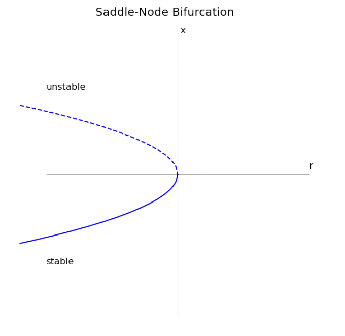
Saddle-Node Bifurcations

Two fixed points collide and annihilate as we modify a parameter

Phase Portrait

Example:

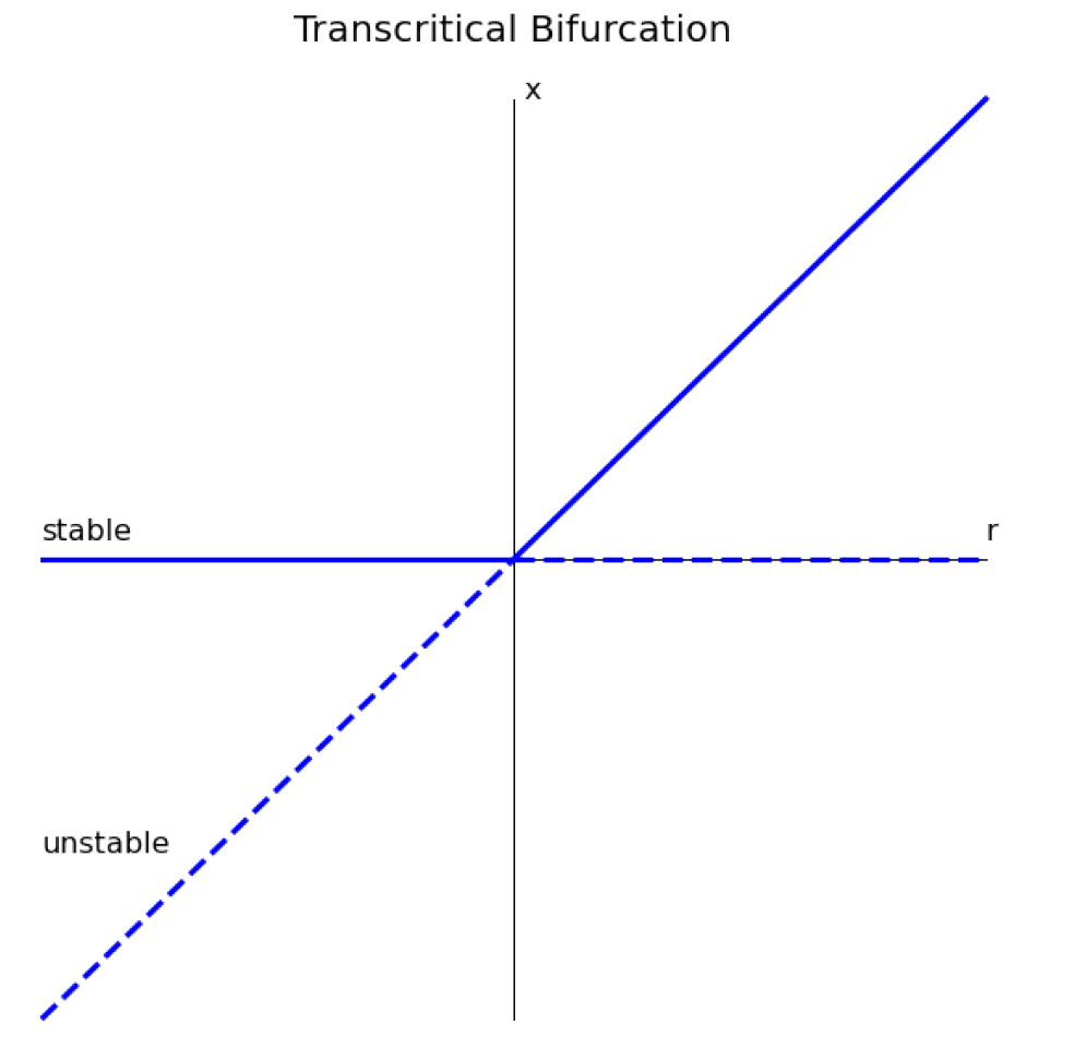
Transcritical Bifurcation

Two fixed points meet and switches stability as a parameter changes

Example:

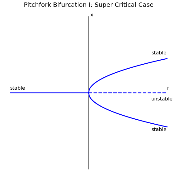
Pitchfork Bifurcation

A fixed point transits into three fixed points as a parameter varies

Super-Critical Pitchfork Bifurcation

Example:

Sub-Critical Pitchfork Bifurcation

Example:

Which would have the a similar diagram as the previous example just flipped over the vertical axis

Hopf Bifurcation

A fixed point loses stability and a periodic solution arises.